Descriptive vs. Inferential Statistics: The Complete Data Science Guide

You have just finished running a customer satisfaction survey. Five hundred responses sit in your dataframe, beautifully cleaned and ready to go. You compute the average rating, build a few histograms, and present the results to your stakeholders. Someone in the back row raises their hand and asks the one question that makes your stomach drop: “How confident are you that this reflects all our customers, not just the 500 who responded?”

If you do not have an answer ready, you have only done half the job.

That is the difference between descriptive and inferential statistics. One summarizes what you see. The other tells you what it means. Most data science curricula teach the formulas, but they do not always teach when to switch from “describing” to “inferring.” Mastering that switch is what separates a dashboard builder from a decision scientist.

The Two Branches: What Happened vs. What It Means

Before any model is built, any hypothesis is tested, or any business decision is made, statistics is already doing the heavy lifting. It breaks down into two foundational branches:

| Branch                     | Core Question                           | Scope                                       |
| -------------------------- | --------------------------------------- | ------------------------------------------- |
| Descriptive Statistics     | What does the data look like?           | Summarizes the data you have                |
| Inferential Statistics     | What can we conclude beyond the data?   | Draws conclusions about a larger population |

Think of it this way: if you survey 500 customers, descriptive statistics summarizes those 500 responses. Inferential statistics uses those 500 responses to make claims about all your customers. You need both. Descriptive stats without inference is a report that goes nowhere. Inference without descriptive stats is a conclusion built on sand.

Part 1: Descriptive Statistics

What Is Descriptive Statistics?

Descriptive statistics is the practice of summarizing, organizing, and presenting data in a meaningful way. It does not attempt to generalize beyond the dataset. It describes only what is directly observed.

Every Exploratory Data Analysis (EDA) pipeline is fundamentally a descriptive statistics exercise. Before you ask “is this difference significant?” you must answer “what does my data even look like?” Skipping this step is one of the most expensive mistakes in data science. You cannot fix what you have not measured, and you cannot model what you do not understand.

A. Measures of Central Tendency

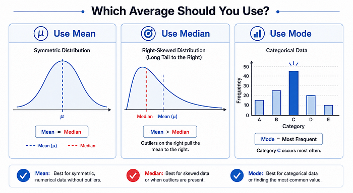
These describe where the “center” of the data lives. They answer the question: what is typical?

source: OpenAI GPT Image 2 model

Mean (Arithmetic Average)

The sum of all values divided by the count of values. We will use these values for the example.

μ = (Σ xᵢ) / n

import numpy as np

data = [12, 15, 14, 10, 18, 22, 14, 16]

mean = np.mean(data)
print(f"Mean: {mean}")  # Output: 15.125

When to use: Continuous data without extreme outliers. The mean is sensitive to outliers. A single extreme value can pull it significantly in one direction.

Example: Average salary in a company. If the CEO earns $5M and all others earn $60K, the mean salary is misleading. It tells you almost nothing about the typical employee.

Median

The middle value when data is sorted. For even-length datasets, it is the average of the two middle values.

median = np.median(data)
print(f"Median: {median}")  # Output: 14.5

When to use: When data is skewed or contains outliers. The median is robust. Extreme values do not affect it, which is why it is the standard for reporting income and house prices.

Example: House prices, income distributions. Always prefer median when the distribution is right-skewed.

Mode

The most frequently occurring value. A dataset can be unimodal, bimodal, or multimodal.

from scipy import stats

mode_result = stats.mode(data, keepdims=True)
print(f"Mode: {mode_result.mode[0]}")  # Output: 14

When to use: Categorical data or discrete distributions. The mode is the only measure of central tendency that makes sense for non-numeric data.

Example: Most common product category purchased, most frequent support ticket type.

Mean vs Median vs Mode: When to Use Which

B. Measures of Dispersion (Spread)

Central tendency only tells half the story. Dispersion describes how spread out the values are around the center. Two datasets can have identical means and look completely different.

Range

The simplest measure: the difference between the maximum and minimum values.

Range = max(x) - min(x)

data_range = np.max(data) - np.min(data)
print(f"Range: {data_range}")  # Output: 12

Limitation: Extremely sensitive to a single outlier. Two datasets can have identical ranges with very different distributions.

Variance

The average of squared deviations from the mean. Squaring removes negatives and penalizes large deviations.

σ² = Σ(xᵢ - μ)² / n           # Population variance
s² = Σ(xᵢ - x̄)² / (n - 1)    # Sample variance (Bessel's correction)

pop_variance  = np.var(data)           # Population (divides by n)
samp_variance = np.var(data, ddof=1)   # Sample (divides by n-1)

print(f"Population Variance: {pop_variance:.2f}")
print(f"Sample Variance:     {samp_variance:.2f}")

Why n-1 for samples? Using n would systematically underestimate the true population variance. Subtracting 1 (Bessel’s correction) produces an unbiased estimate.

Standard Deviation

The square root of variance. It brings units back to the same scale as the original data, making it interpretable.

σ = √(Σ(xᵢ - μ)² / n)

std_dev = np.std(data, ddof=1)  # Sample standard deviation
print(f"Std Dev: {std_dev:.2f}")

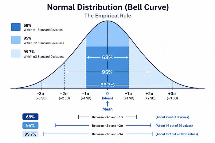
Interpretation rule of thumb (Normal distribution):

• ~68% of data falls within ±1σ of the mean
• ~95% of data falls within ±2σ of the mean
• ~99.7% of data falls within ±3σ of the mean

This is the 68–95–99.7 rule, and it is why standard deviation is the go-to measure of spread for roughly normal data.

Interquartile Range (IQR)

The range of the middle 50% of the data. Computed as Q3 minus Q1.

IQR = Q3 - Q1    (75th percentile - 25th percentile)

Q1  = np.percentile(data, 25)
Q3  = np.percentile(data, 75)
IQR = Q3 - Q1

print(f"Q1: {Q1}, Q3: {Q3}, IQR: {IQR}")

# Outlier detection using IQR fences
lower_fence = Q1 - 1.5 * IQR
upper_fence = Q3 + 1.5 * IQR
outliers = [x for x in data if x < lower_fence or x > upper_fence]
print(f"Outliers: {outliers}")

IQR is the standard method for outlier detection in box plots and most preprocessing pipelines. Unlike range and standard deviation, it is not influenced by extreme values.

C. Measures of Shape

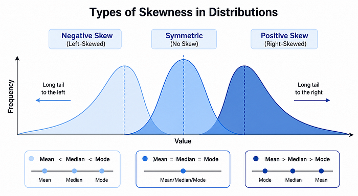
Skewness

Measures the asymmetry of the distribution.

from scipy.stats import skew

skewness = skew(data)
print(f"Skewness: {skewness:.3f}")

| Skewness Value | Shape                   | Tail direction  | Mean vs Median |
| -------------- | ----------------------- | --------------- | -------------- |
| skew ≈ 0       | Symmetric               | Balanced        | Mean ≈ Median  |
| skew > 0       | Right-skewed (positive) | Long right tail | Mean > Median  |
| skew < 0       | Left-skewed (negative)  | Long left tail  | Mean < Median  |

Practical implication: Income data is typically right-skewed. Log transformation is commonly applied to normalize it before modeling.

Kurtosis

Measures the “tailedness” of the distribution: how heavy or light the tails are relative to a normal distribution.

from scipy.stats import kurtosis

kurt = kurtosis(data)  # Excess kurtosis (relative to normal = 0)
print(f"Kurtosis: {kurt:.3f}")

| Kurtosis       | Type        | Tails                   |
| -------------- | ----------- | ----------------------- |
| = 0 (excess)   | Mesokurtic  | Normal-like tails       |
| > 0 (excess)   | Leptokurtic | Heavy tails, sharp peak |
| < 0 (excess)   | Platykurtic | Light tails, flat peak  |

Practical implication: Financial return data is typically leptokurtic. Fat tails mean extreme events happen more often than a normal distribution predicts. This is critical for risk modeling.

Five-Number Summary

The five-number summary compactly describes any distribution:

Minimum | Q1 | Median (Q2) | Q3 | Maximum

import pandas as pd

df = pd.DataFrame(data, columns=["value"])
print(df["value"].describe())

This single line gives you quick descriptive analysis of a dataset: count, mean, standard deviation, min, quartiles, and max. It is the fastest sanity check you can run on any numeric column.

Here is an example of end-to-end code pipeline for all of the concepts of descriptive statistics, you may copy them to Google Colab to quick check the result.

"""
descriptive_statistics.py

A comprehensive demonstration of descriptive statistics using NumPy, SciPy, and Pandas.
Covers central tendency, dispersion, shape measures, and the five-number summary.
"""

import numpy as np
import pandas as pd
from scipy import stats

# ---------------------------------------------------------------------------
# Sample data: customer purchase amounts in dollars
# ---------------------------------------------------------------------------
data = [12, 15, 14, 10, 18, 22, 14, 16]

print("=" * 60)
print("DESCRIPTIVE STATISTICS DEMONSTRATION")
print("=" * 60)

# ---------------------------------------------------------------------------
# 1. Measures of Central Tendency
# ---------------------------------------------------------------------------
print("\n--- Measures of Central Tendency ---\n")

# Mean (arithmetic average)
mean = np.mean(data)
print(f"Mean:   {mean:.3f}")

# Median (middle value)
median = np.median(data)
print(f"Median: {median:.3f}")

# Mode (most frequent value)
mode_result = stats.mode(data, keepdims=True)
print(f"Mode:   {mode_result.mode[0]}")

# ---------------------------------------------------------------------------
# 2. Measures of Dispersion (Spread)
# ---------------------------------------------------------------------------
print("\n--- Measures of Dispersion ---\n")

# Range: max - min
data_range = np.max(data) - np.min(data)
print(f"Range:              {data_range}")

# Variance: population vs sample
pop_variance = np.var(data)          # Population (divides by n)
samp_variance = np.var(data, ddof=1) # Sample (divides by n-1)
print(f"Population Variance: {pop_variance:.3f}")
print(f"Sample Variance:     {samp_variance:.3f}")

# Standard Deviation: square root of variance
std_dev = np.std(data, ddof=1)  # Sample standard deviation
print(f"Sample Std Dev:      {std_dev:.3f}")

# Interquartile Range (IQR): Q3 - Q1
Q1 = np.percentile(data, 25)
Q3 = np.percentile(data, 75)
IQR = Q3 - Q1
print(f"Q1: {Q1}, Q3: {Q3}, IQR: {IQR}")

# Outlier detection using IQR fences
lower_fence = Q1 - 1.5 * IQR
upper_fence = Q3 + 1.5 * IQR
outliers = [x for x in data if x < lower_fence or x > upper_fence]
print(f"Lower Fence: {lower_fence:.2f}, Upper Fence: {upper_fence:.2f}")
print(f"Outliers: {outliers}")

# ---------------------------------------------------------------------------
# 3. Measures of Shape
# ---------------------------------------------------------------------------
print("\n--- Measures of Shape ---\n")

# Skewness: asymmetry of the distribution
skewness = stats.skew(data)
print(f"Skewness:  {skewness:.3f}")
if skewness > 0.5:
    print("  -> Distribution is right-skewed (positive)")
elif skewness < -0.5:
    print("  -> Distribution is left-skewed (negative)")
else:
    print("  -> Distribution is approximately symmetric")

# Kurtosis: tailedness relative to normal distribution
kurt = stats.kurtosis(data)  # Excess kurtosis
print(f"Kurtosis:  {kurt:.3f}")
if kurt > 0:
    print("  -> Leptokurtic: heavy tails, sharp peak")
elif kurt < 0:
    print("  -> Platykurtic: light tails, flat peak")
else:
    print("  -> Mesokurtic: normal-like tails")

# ---------------------------------------------------------------------------
# 4. Five-Number Summary using Pandas
# ---------------------------------------------------------------------------
print("\n--- Five-Number Summary ---\n")

df = pd.DataFrame(data, columns=["purchase_amount"])
summary = df["purchase_amount"].describe()
print(summary)

print("\n" + "=" * 60)

Part 2: Inferential Statistics

What Is Inferential Statistics?

Inferential statistics uses a sample to make probabilistic conclusions about a larger population. Because collecting data on an entire population is usually impossible, we rely on sampling and probability theory to estimate population parameters and test hypotheses.

The central challenge is this: how confident can we be that our sample reflects the truth about the population? Inferential statistics gives you the tools to answer that question with mathematical rigor.

Populations and Samples

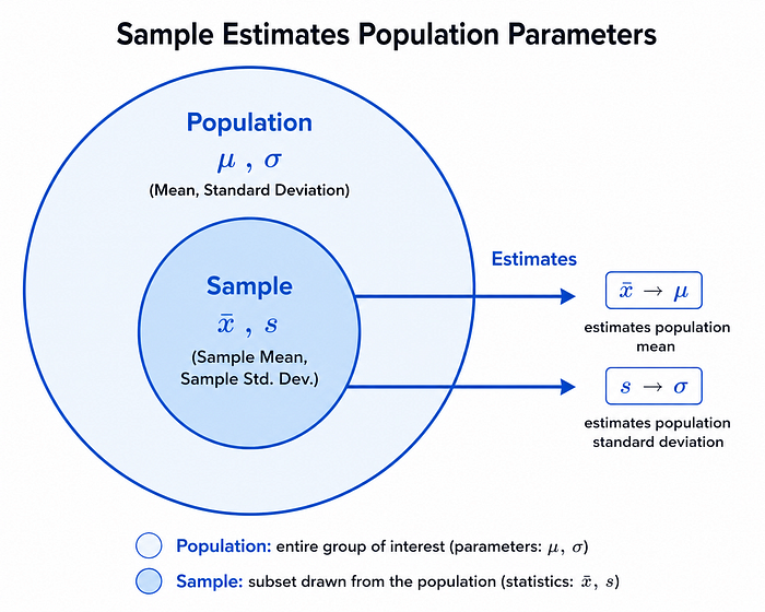
| Concept            | Symbol (Population) | Symbol (Sample) | Description              |
| ------------------ | ------------------- | --------------- | ------------------------ |
| Mean               | μ (mu)              | x̄ (x-bar)      | Average                  |
| Standard Deviation | σ (sigma)           | s               | Spread                   |
| Proportion         | p                   | p̂ (p-hat)      | Fraction with a property |
| Size               | N                   | n               | Number of observations   |

Key principle: Sample statistics (x̄, s, p̂) are used as estimators of unknown population parameters (μ, σ, p). Inferential statistics quantifies how good those estimates are.

The Central Limit Theorem

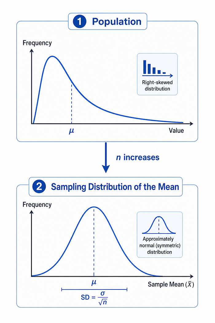
One of the most powerful results in statistics:

Regardless of the shape of the population distribution, the sampling distribution of the sample mean approaches a normal distribution as sample size increases, provided n is sufficiently large (typically n ≥ 30).

x̄ ~ N(μ, σ²/n)

Standard Error (SE) = σ / √n

import numpy as np
import matplotlib.pyplot as plt

# Simulate CLT: draw from a skewed (exponential) distribution
population = np.random.exponential(scale=2, size=100_000)
sample_means = [np.mean(np.random.choice(population, size=50)) for _ in range(5000)]

# sample_means is approximately normally distributed
print(f"Mean of sample means: {np.mean(sample_means):.3f}")
print(f"Std of sample means (SE): {np.std(sample_means):.3f}")

Why it matters: The CLT is what makes most inferential procedures valid in practice, even when population distributions are unknown or non-normal. It is the reason a data scientist can trust a t-test on skewed website latency data.

Confidence Intervals

A confidence interval (CI) provides a range of plausible values for a population parameter, along with a confidence level expressing how reliable that range is.

CI = x̄ ± (critical_value × SE)

Where SE = s / √n

import scipy.stats as stats
import numpy as np

sample = np.array([12, 15, 14, 10, 18, 22, 14, 16, 19, 13])
n      = len(sample)
x_bar  = np.mean(sample)
se     = stats.sem(sample)          # Standard error of the mean

# 95% confidence interval using t-distribution (small sample)
ci_lower, ci_upper = stats.t.interval(
    confidence=0.95,
    df=n - 1,
    loc=x_bar,
    scale=se
)
print(f"Sample Mean: {x_bar:.2f}")
print(f"95% CI: ({ci_lower:.2f}, {ci_upper:.2f})")

Correct Interpretation (Important!)

We are 95% confident that the true population mean falls between ci_lower and ci_upper.

Common misconception: A 95% CI does NOT mean there is a 95% probability the true parameter is in this specific interval. The parameter is fixed. The interval is random. If you repeated the experiment 100 times, approximately 95 of those intervals would contain the true parameter.